Data Analysis using SQL – Part 3 – Advanced SQL

You now know two types of SQL commands, namely:
- Data Definition Language
- Data Manipulation Language
The Data Definition Language (DDL) is used to create and modify the schema of the database. Commands like CREATE, ALTER and DROP are part of this language.
As a data analyst, you would always be actively involved in data retrieval activities. Here, the Data Manipulation Language (DML) commands would come in handy, e.g. the DML command SELECT, its purpose, various clauses and filtering operations.
Order by Clause
The SQL ORDER BY clause is used to sort the data in ascending or descending order, based on one or more columns. Some databases sort the query results in an ascending order by default.
The basic syntax of the ORDER BY clause is as follows −
SELECT column-list
FROM table_name
[WHERE condition]
[ORDER BY column1, column2, .. columnN] [ASC | DESC];
The order in which it appears is “select * from table where some_variable = x order by some_variable”.
Example
SELECT *
FROM CUSTOMERS
WHERE AGE >32
ORDER BY NAME, SALARY;
Aggregate Functions
An SQL aggregate function calculates on a set of values and returns a single value. For example, the average function ( AVG) takes a list of values and returns the average.
The following are the commonly used SQL aggregate functions:
-
AVG()– returns the average of a set. -
COUNT()– returns the number of items in a set. -
MAX()– returns the maximum value in a set. -
MIN()– returns the minimum value in a set -
SUM()– returns the sum of all or distinct values in a set
Except for the COUNT() function, SQL aggregate functions ignore null.
You can use aggregate functions as expressions only in the following:
- The select list of a
SELECTstatement, either a subquery or an outer query. - A
HAVINGclause
Group by Clause
Many times as an analyst, you would have to generate reports related to specific departments. In such scenarios, you would collect information on departments, products, assembly lines, vendors, etc. SQL provides a special clause called ‘Group by’ for collecting facts about certain categories.
The SQL GROUP BY clause is used in collaboration with the SELECT statement to arrange identical data into groups. This GROUP BY clause follows the WHERE clause in a SELECT statement and precedes the ORDER BY clause.
The basic syntax of a GROUP BY clause is shown in the following code block. The GROUP BY clause must follow the conditions in the WHERE clause and must precede the ORDER BY clause if one is used.
SELECT column1, column2
FROM table_name
WHERE [ conditions ]
GROUP BY column1, column2
ORDER BY column1, column2
Example
SELECT COUNT(CustomerID), Country
FROM Customers
GROUP BY Country;
Having Clause
Suppose your manager asks you to count all the employees whose salary is more than the average salary in that particular department. Now, intuitively, you know that two aggregate functions would be used here — count() and avg(). You decide to apply the where condition on the average salary of the department, but to your surprise, the query fails. In fact, you should try writing this query before moving ahead.
The HAVING Clause enables you to specify conditions that filter which group results appear in the results.
The WHERE clause places conditions on the selected columns, whereas the HAVING clause places conditions on groups created by the GROUP BY clause.
The following code block shows the position of the HAVING Clause in a query.
SELECT column1, column2
FROM table1, table2
WHERE [ conditions ]
GROUP BY column1, column2
HAVING [ conditions ]
ORDER BY column1, column2
Example
SELECT ID, NAME, AGE, ADDRESS, SALARY
FROM CUSTOMERS
GROUP BY age
HAVING COUNT(age) >= 2;
The having clause is typically used when you have to apply a filter condition on an ‘aggregated value’. This is because the ‘where’ clause is applied before the aggregation takes place, and thus it is not useful when you want to apply a filter on an aggregated value.
In other words, the having clause is equivalent to a where clause after the group by has been executed but before the select part is executed.
Nested Queries
You know that a database is a collection of multiple related tables. While generating insights from the data, you may need to refer to these multiple tables in a query. There are two ways to deal with such types of queries:
- Joins
- Nested queries/Subqueries
A subquery is used to return data that will be used in the main query as a condition to further restrict the data to be retrieved.
Subqueries can be used with the SELECT, INSERT, UPDATE, and DELETE statements along with the operators like =, <, >, >=, <=, IN, BETWEEN, etc.
There are a few rules that subqueries must follow −
- Subqueries must be enclosed within parentheses.
- A subquery can have only one column in the SELECT clause, unless multiple columns are in the main query for the subquery to compare its selected columns.
- An ORDER BY command cannot be used in a subquery, although the main query can use an ORDER BY. The GROUP BY command can be used to perform the same function as the ORDER BY in a subquery.
- Subqueries that return more than one row can only be used with multiple value operators such as the IN operator.
- The SELECT list cannot include any references to values that evaluate to a BLOB, ARRAY, CLOB, or NCLOB.
- A subquery cannot be immediately enclosed in a set function.
- The BETWEEN operator cannot be used with a subquery. However, the BETWEEN operator can be used within the subquery.
Subqueries with the SELECT Statement
Subqueries are most frequently used with the SELECT statement. The basic syntax is as follows −
SELECT column_name [, column_name ]
FROM   table1 [, table2 ]
WHERE  column_name OPERATOR
   (SELECT column_name [, column_name ]
   FROM table1 [, table2 ]
   [WHERE])
Inner Join
The most important and frequently used of the joins is the INNER JOIN. They are also referred to as an EQUIJOIN.
The INNER JOIN creates a new result table by combining column values of two tables (table1 and table2) based upon the join-predicate. The query compares each row of table1 with each row of table2 to find all pairs of rows which satisfy the join-predicate. When the join-predicate is satisfied, column values for each matched pair of rows of A and B are combined into a result row.
Syntax
The basic syntax of the INNER JOIN is as follows.
SELECT table1.column1, table2.column2...
FROM table1
INNER JOIN table2
ON table1.common_field = table2.common_field;
Example
SELECT  ID, NAME, AMOUNT, DATE
   FROM CUSTOMERS
   INNER JOIN ORDERS
   ON CUSTOMERS.ID = ORDERS.CUSTOMER_ID;
Multi Join
Multi-joins, you can join multiple tables using the common attributes between pairs of tables. This is possible because the result of a join is also a table which you can join further to another table (with a common attribute).
Example
SELECT customerName, customercity, customermail, salestotal
FROM onlinecustomers AS oc
   INNER JOIN
   orders AS o
   ON oc.customerid = o.customerid
   INNER JOIN
   sales AS s
   ON o.orderId = s.orderId
Outer Join
In an inner join, all the records from the first table are referred to and joined together. However, there may be situations when you need to join the records based on a second table.
There are three kinds of OUTER JOIN: left outer join, right outer join and full outer join. Let’s examine each kind of join in more detail.
SQL OUTER JOIN – left outer join
SQL left outer join is also known as SQL left join. Suppose, we want to join two tables: A and B. SQL left outer join returns all rows in the left table (A) and all the matching rows found in the right table (B). It means the result of the SQL left join always contains the rows in the left table.
The following illustrate SQL left outer syntax of joining 2 tables: table_A and table_B:
| 1234 | SELECT column1, column2… FROM table_ALEFT JOIN table_B ON join_conditionWHERE row_condition |
SQL OUTER JOIN – left outer join example
The following query selects all customers and their orders:
| 123456 | SELECT c.customerid, c.companyName, orderidFROM customers cLEFT JOIN orders o ON o.customerid = c.customeridORDER BY orderid |
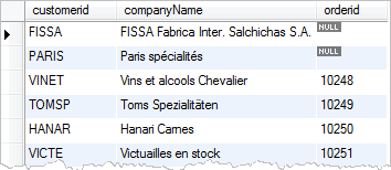
All rows in the customers table are listed. In case, there is no matching row in the orders table found for the row in the customers table, the orderid column in the orders table is populated with NULL values.
We can use Venn diagram to visualize how SQL LEFT OUTER JOIN works.
SQL OUTER JOIN – right outer join
SQL right outer join returns all rows in the right table and all the matching rows found in the left table. The syntax of the SQL right outer join is as follows:
| 1234 | SELECT column1, column2… FROM table_ARIGHT JOIN table_B ON join_conditionWHERE row_condition |
SQL right outer join is also known as SQL right join.
SQL OUTER JOIN – right outer join example
The following example demonstrates the SQL right outer join:
| 123456 | SELECT c.customerid, c.companyName, orderidFROM customers cRIGHT JOIN orders o ON o.customerid = c.customeridORDER BY orderid |
The query returns all rows in the orders table and all matching rows found in the customers table.
The following Venn diagram illustrates how the SQL right outer join works:
SQL OUTER JOIN – full outer join
The syntax of the SQL full outer join is as follows:
| 1234 | SELECT column1, column2… FROM table_AFULL OUTER JOIN table_B ON join_conditionWHERE row_condition |
SQL full outer join returns:
- all rows in the left table table_A.
- all rows in the right table table_B.
- and all matching rows in both tables.
Some database management systems do not support SQL full outer join syntax e.g., MySQL. Because SQL full outer join returns a result set that is a combined result of both SQL left join and SQL right join. Therefore you can easily emulate the SQL full outer join using SQL left join and SQL right join with UNION operator as follows:
| 1234567 | SELECT column1, column2… FROM table_ALEFT JOIN table_B ON join_conditionUNIONSELECT column1, column2… FROM table_ARIGHT JOIN table_B ON join_condition |
SQL OUTER JOIN – full outer join example
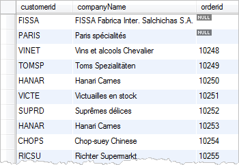
The following query demonstrates the SQL full outer join:
| 123456 | SELECT c.customerid, c.companyName, orderidFROM customers cFULL OUTER JOIN orders o ON o.customerid = c.customeridORDER BY orderid |
The following Venn diagram illustrates how SQL full outer join works:
I
What is the difference between “INNER JOIN” and “OUTER JOIN”?
Assuming you’re joining on columns with no duplicates, which is a very common case:
- An inner join of A and B gives the result of A intersect B, i.e. the inner part of a Venn diagram intersection.
- An outer join of A and B gives the results of A union B, i.e. the outer parts of a Venn diagram union.
Examples
Suppose you have two tables, with a single column each, and data as follows:
A    B
-    -
1    3
2    4
3    5
4    6
Note that (1,2) are unique to A, (3,4) are common, and (5,6) are unique to B.
Inner join
An inner join using either of the equivalent queries gives the intersection of the two tables, i.e. the two rows they have in common.
select * from a INNER JOIN b on a.a = b.b;
select a.*, b.*  from a,b where a.a = b.b;

a | b
--+--
3 | 3
4 | 4
Left outer join
A left outer join will give all rows in A, plus any common rows in B.
select * from a LEFT OUTER JOIN b on a.a = b.b;
select a.*, b.*  from a,b where a.a = b.b(+);

a |  b
--+-----
1 | null
2 | null
3 |    3
4 |    4
Right outer join
A right outer join will give all rows in B, plus any common rows in A.
select * from a RIGHT OUTER JOIN b on a.a = b.b;
select a.*, b.*  from a,b where a.a(+) = b.b;

a    |  b
-----+----
3    |  3
4    |  4
null |  5
null |  6
Full outer join
A full outer join will give you the union of A and B, i.e. all the rows in A and all the rows in B. If something in A doesn’t have a corresponding datum in B, then the B portion is null, and vice versa.
select * from a FULL OUTER JOIN b on a.a = b.b;

 a   |  b
-----+-----
   1 | null
   2 | null
   3 |    3
   4 |    4
null |    6
null |    5
Summary
We began this session with a discussion on the ‘Order by’ clause. This clause is used to order the records retrieved through a query. The ‘order by’ clause has a constraint in that it is always the last clause in any query.
The session also covered grouped aggregation and other aggregation functions. You learnt the ‘group by’ and other aggregation functions such as max(), min(), count(), etc. The ‘where’ clause can’t be used on aggregate functions, so the ‘having’ clause comes handy here.
Both “Having” and “Where” clauses are similar in nature and have a functionality of “FILTERING” the data with a slight difference. The WHERE clause filters on individual rows and the HAVING clause filters on the aggregated values, it applies only to groups as a whole.
Further, the session covered the concepts of nested queries and joins, including inner join, outer join, left outer join, right outer join, among others.